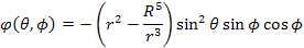
1. A conducting sphere of radius R is kept in an electrostatic field given by  . Obtain an expression for the potential in the region outside the sphere and obtain the charge density on the sphere

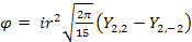
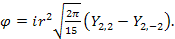
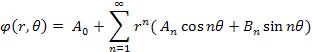
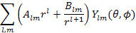
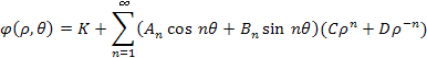
The potential corresponding to the electric field is . Using the table for Spherical harmonics, the potential can be expressed as  The general expression for solution of Laplace’s equation is

The boundary conditions to be satisfied are :

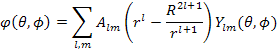
(i) For all , for , the potential is constant, which we take to be zero. This implies  for all m. This makes the potential expression to be

(ii )For large distances, , .  in this limit,, the second term for the expression for potential goes to zero and we are left with,

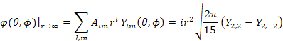
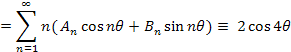
Comparing, we get only non-zero value of to be 2 and the corresponding m values as . Thus, the potential has the form

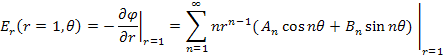
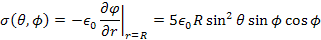
The surface charge density is given by

2.A unit disk  has no sources of charge on it. The electric field on the rim  is given by , where  is the polar angle. Obtain an expression for potential inside the disk.

The solution of Laplace’s equation on a unit disk is given by (see tutorial problem)

The electric field is given by the negative gradient of potential. Since the field is given to be radial,

This gives all coefficients other than  to be zero and  The coefficient  , however remains undetermined.

3. (Hard Problem) A cylindrical conductor of infinite length  has its curved surfaces divided into two equal halves, the part with polar angle  has a constant potential  while the remaining half is at a potential . Obtain an expression  for the potential inside the cylinder. Verify your result by calculating the potential on the surface at  and at .

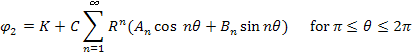
Because of symmetry along the z axis, the potential can only depend on the polar coordinates .  By using a separation of variables, we can show, as shown in the lecture, the angular part  The radial equation has the solution , we have ignored n=0 solution because it gives rise to logarithm in radial coordinate which diverges at origin. Thus the general solution for the potential is

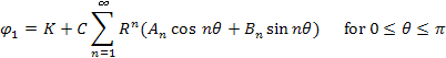
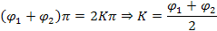
where  K is a constant.  Further, the constant D must be zero otherwise the potential would diverge at . Let us now apply the boundary conditions,  For

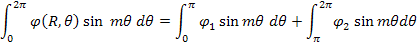
Integrate the first expression from  and the second expression from  and add. The integration over the second term on the right hand side of the two expressions is equal to an integration from 0 to 2p and the integral vanishes.  We are left with

Thus the potential expression at  becomes

            (I)
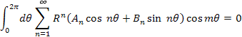
To evaluate the coefficients , multiply both sides by  and integrate from 0 to 2p,
L.H.S. gives,

Similarly, the first term on the right also gives zero.
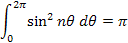
We are left with

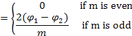
These integrals can be done by elementary methods,
If

If ,

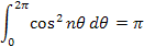
Thus,
 
To determine the coefficients , multiply both sides of  (I) by   and integrate from 0 to 2p,
L.H.S. gives,

The first term on the right gives zero.
We are left with

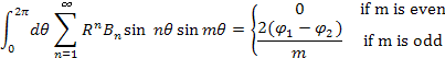
The integral can be easily done If

If ,

Thus,

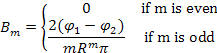
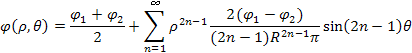
Let us write,
We have the final expression for the potential,

 

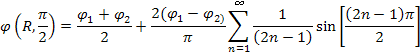
To verify that this is consistent with the given boundary conditions, let us evaluate the potential at ,

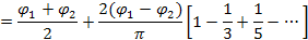
The infinite series has a value . Adding , we get . Similarly, one can check that .